The Labor Market
Introduction
This example builds a demand and supply of labor. The former is derived from a firms profit maximization problem. The latter from a consumer utility maximization problem. The example also calculates and plots the equilibrium of the labor market.
Labor demand
Labor demand $\left(N^D\right)$ originates in a representative firm maximizing its profits $(\pi)$. Assume output $(Q)$ follows a Cobb-Douglas production function with Hicks-Neutral technology $(A)$, and that $P$ is the market price of the firm’s output. Further, assume that $w$ and $r$ are the prices of labor $(N)$ and capital $(K)$ respectively. Then, firm’s profit is (where $\alpha \in (0, 1)$):
$$ \begin{align} \pi &= P \cdot Q(K, N) - wN - rK \\[10pt] \pi &= P \cdot \left(A K^{\alpha} N^{1-\alpha} \right) - wN - rK \end{align} $$
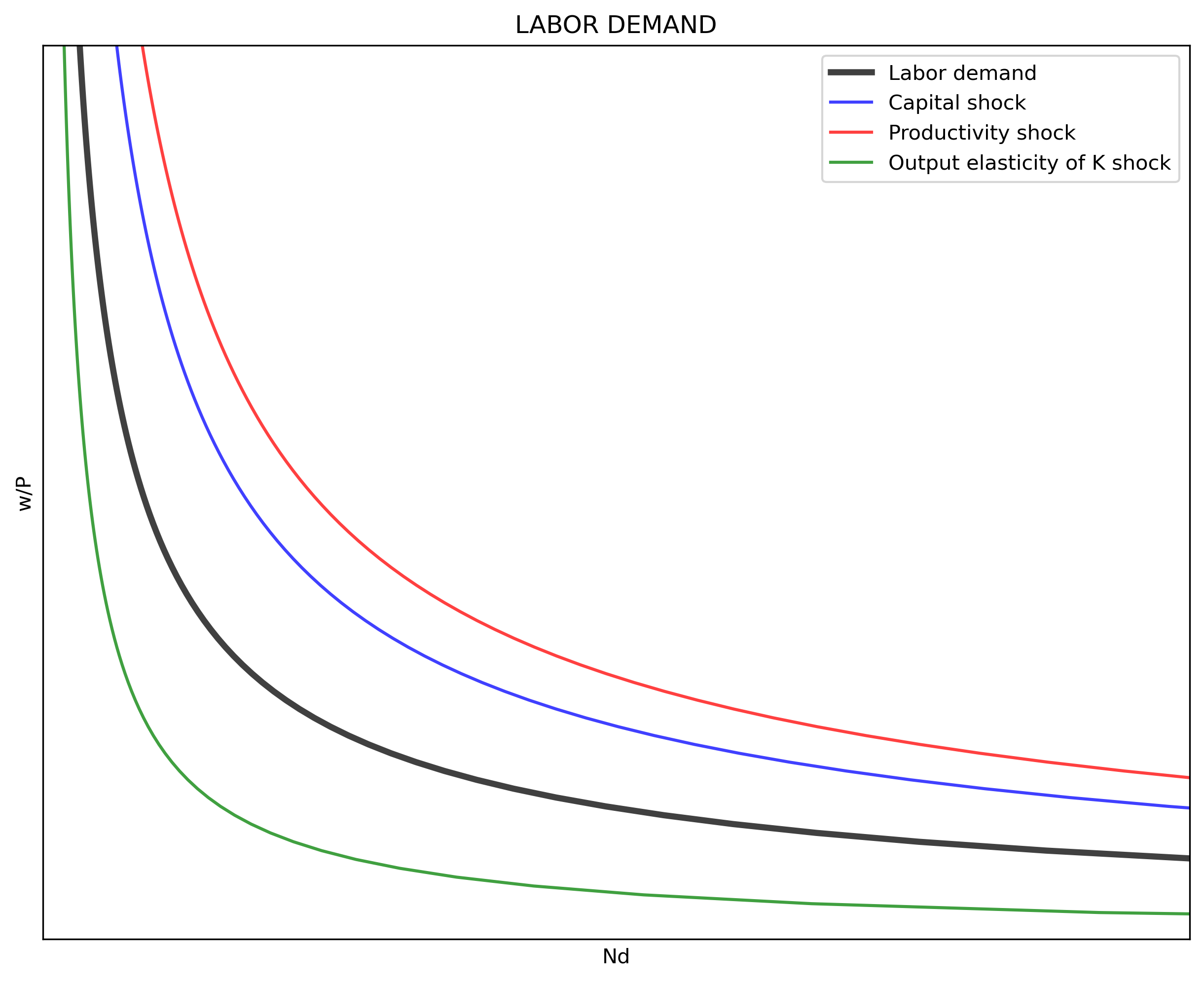
With capital and technology fixed in the short-run, the firm maximizes its profits by changing the amount of labor. The firm demands labor (that has decreasing marginal returns) up the points of its marginal productivity. It can be seen that labor demand has an hyperbolic shape with respect to real wages $(w/P)$.
$$ \begin{align} \frac{\partial \pi}{\partial N} &= P \cdot (1-\alpha) A \left(\frac{K}{N}\right)^{\alpha} - w= 0 \\[10pt] N^D &= K \cdot \left[\frac{(1-\alpha)A}{(w/P)}\right]^{1/\alpha} \end{align} $$
The following code plots labor demand and shifts produced by changes in $K$ (in blue), $A$ (in red), and in $\alpha$ (in green). The first part of the code imports the required packages. The second part defines the parameters and vectors to be used. The third part of the code builds the labor demand function. The fourth section calculates labor demand and the effects of shocks (1) to capital $(\Delta K = 20)$, (2) to productivity $(\Delta A = 20)$, and (3) to output elasticity of capital $(\Delta \alpha = 20)$. The fifth part of the code plots labor demand and the shock effects.
#%% | *** CELL 1 ***
"============================================================================"
"1|IMPORT PACKAGES"
import numpy             as np       # Package for scientific computing
import matplotlib.pyplot as plt      # Matplotlib is a 2D plotting library
from   scipy.optimize    import root # Package to find the roots of a function


"============================================================================"
"2|DEFINE PARAMETERS AND ARRAYS"
# Code parameters
dpi=300
size  = 50    # Real wage domain
# Model parameters
K     = 20    # Capital stock
A     = 20    # Technology
alpha =  0.7  # Output elasticity of capital
# Arrays
rW = np.linspace(1, size, size*2)  # Real wage


"============================================================================"
"3|LABOR DEMAND FUNCTION"
def Ndemand(A, K, rW, alpha):
    Nd = K * ((1 - alpha)*A/rW)**(1/alpha)
    return Nd


"============================================================================"
"4|CALCULATE LABOR DEMAND AND SHOCK EFFECTS"
D_K = 20    # Shock to K
D_A = 20    # Shock to A
D_a =  0.2  # Shock to alpha

Nd   = Ndemand(A    , K    , rW, alpha)
Nd_K = Ndemand(A    , K+D_K, rW, alpha)
Nd_A = Ndemand(A+D_A, K    , rW, alpha)
Nd_a = Ndemand(A    , K    , rW, alpha+D_a)


"============================================================================"
"5|PLOT LABOR DEMAND AND SHOCK EFFECTS"
# AXIS RANGE
axis_range = [0, 30, 0, size]

# BUILD PLOT
fig, ax = plt.subplots(figsize=(10, 8), dpi=dpi)
ax.set(title="LABOR DEMAND", xlabel=r'Nd', ylabel=r'w/P')
# ADD DEMAND CURVES
ax.plot(Nd  , rW, "k-", alpha=0.75, label="Labor demand", linewidth=3)
ax.plot(Nd_K, rW, "b-", alpha=0.75, label="Capital shock")
ax.plot(Nd_A, rW, "r-", alpha=0.75, label="Productivity shock")
ax.plot(Nd_a, rW, "g-", alpha=0.75, label="Output elasticity of K shock")
# AXIS
ax.yaxis.set_major_locator(plt.NullLocator())   # Hide ticks
ax.xaxis.set_major_locator(plt.NullLocator())   # Hide ticks
#SETTINGS
ax.grid()
ax.legend()
plt.axis(axis_range)
plt.show()
Labor supply
Labor supply is derived from the consumer maximizing a constrained utility function. The consumer receives utility from consumption $(C)$ and leisure time $(L)$. While the profit function of the firm has an internal maximum, the utility function is strictly increasing on $C$ and $L$. Put it differently, there is a point after which increasing output does not increase profits. But, utility always increases (even if by a very small amount) with more consumption. Therefore, the utility maximization problem includes (1) a binding constrain and (2) the right mix of $C$ and $L$ that will depend on their relative prices.
Assume a Cobb-Douglas utility function where $\beta$ is the consumption elasticity of utility.
$$ \begin{equation} U(C, L) = C^{\beta} L^{1-\beta} \end{equation} $$
The consumer faces the following budget constraint:
$$ \begin{align} C &= \left(\frac{w}{P} \right) (T - L) + I \\[10pt] C &= \underbrace{\left[I + T \left(\frac{w}{P} \right) \right]}_{\text{intercept}} - \underbrace{\left( \frac{w}{P} \right)}_{\text{slope}}L \end{align} $$
where $T$ is the amount of hours the individual can work in given day and $I$ is other (non-labor) income.
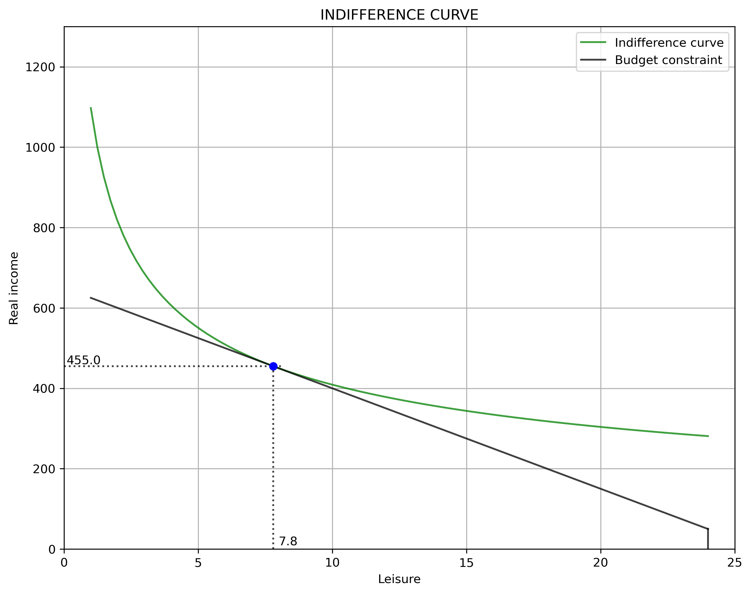
Before deriving labor supply $N^S$ we can plot the indifference curve between consumption and leisure with the budget constraint. “Solving” for $C$ for a given level of utility:
$$ \begin{equation} C = \left(\frac{\bar{U}}{L^{1 - \beta}} \right)^{(1/\beta)} \end{equation} $$
We can now maximize the utility with the budget constraint using a Lagrangian $\left(\Im\right)$:
$$ \begin{equation} \max_{{C, L}} \Im = C^{\beta} L^{1 - \beta} + \lambda \left[C - I - \frac{w}{P} (T - L) \right] \end{equation} $$
The FOC for $\Im$:
$$ \begin{cases} \Im_{L} = (1 - \beta) \left( \frac{C}{L} \right)^{\beta} - \lambda = 0 \\[10pt] \Im_{C} = \beta \left( \frac{L}{C} \right)^{1-\beta} - \lambda \left(\frac{w}{P} \right) = 0 \\[10pt] \Im_{\lambda} = C - I - \left(\frac{w}{P}\right) (T - L) = 0 \end{cases} $$
From the first two FOCs we get the known relationship $\frac{U_{L}}{U_{C}} = \frac{w/P}{1}$
Solving for $C$ in terms of $L$ yields $C = \frac{\beta}{1-\beta} \left(\frac{w}{P}\right)L$. Plugin this result in the third FOC and solving for $L$ yields $L^* = (1-\beta) \left[\frac{I + T (w/P)}{(w/P)} \right]$. With $L^*$ we can now get $C^* = \beta \left[I + T (w/P) \right]$. Next we plug-in $C^*$ and $L^*$ into the utility function.
$$ \begin{align} U^*(C^*, L^*) &= \left(C^* \right)^{\beta} \left(L^* \right)^{1-\beta} \\[10pt] U^*(C^*, L^*) &= \left[\beta(I + T (w/P)\right]^{\beta} \left[(1 - \beta) \frac{I + T(w/P)}{(w/P)} \right]^{1-\beta} \end{align} $$
Using the lagrangian method also allows to find the “optimal” value of $\lambda$ or the “shadow price”:
$$ \begin{align} \lambda^* &= (1-\beta) \left(\frac{C^*}{L^*} \right)^{\beta} \\[10pt] \lambda^* &= (1-\beta) \left[\frac{\beta \left(I+24(w/P)\right)w}{(1-\beta)(I+24(w/P)} \right]^{\beta} \\[10pt] \lambda^* &= (1-\beta) \left(\frac{\beta}{1-\beta} \frac{w}{P} \right)^{\beta} \end{align} $$
Now we can use this information to plot the indifference curve with matplotlib. Note that at $T=24$ (zero hours of labor), income equals $I$ (non-labor income). This shows as a vertical line that connects with the budget constraint, which starts to grow as hours of labor are added.(moving to the left).
#%% *** CELL 2 ***
"============================================================================"
"6|DEFINE PARAMETERS AND ARRAYS"
# Model parameters
T    = 24    # Available hours to work
beta =  0.7  # Utility elasticity of consumption
I    = 50    # Non-labor income
rW2  = 25    # Real wage
# Arrays
L = np.linspace(1, T, T*4)  # Array of labor hours from 0 to T


"============================================================================"
"7|CALCULATE OPTIMAL VALUES AND DEFINE FUNCTIONS"
Ustar = (beta*(I + T*rW2))**beta * ((1 - beta)*(I + T*rW2)/rW2)**(1 - beta)
Lstar = (1 - beta)*((I + T*rW2)/rW2)
Cstar = beta*(I + T*rW2)

# Consumption function
def C_indiff(U, L, beta):
    C_indiff = (U/L**(1 - beta))**(1/beta)
    return C_indiff

# Budget constraint
def Budget(I, rW2, L):
    Budget = (I + T*rW2) - rW2*L
    return Budget

# Populate the indifference curve and the budget constraint
B = Budget(I, rW2, L)
C = C_indiff(Ustar, L, beta)


"============================================================================"
"8|PLOT THE INDIFFERENCE CURVE AND THE BUDDGET CONSTRAINT"
y_max = 2*Budget(I, rW2, 0)

# AXIS RANGE
axis_range = [0, T+1, 0, y_max]

# BUILD PLOT
fig, ax = plt.subplots(figsize=(10, 8), dpi=dpi)
ax.set(title="INDIFFERENCE CURVE", xlabel="Leisure", ylabel="Real income")
# ADD LINES TO THE PLOT
ax.plot(L, C, "g-", alpha=0.75, label="Indifference curve")
ax.plot(L, B, "k-", alpha=0.75, label="Budget constraint")
plt.axvline(x=T    , ymin=0, alpha=0.75, ymax=I/y_max, color='k') # Add I
plt.axvline(x=Lstar, ymin=0, alpha=0.75, ymax = Cstar/y_max, ls=':', color='k')
plt.axhline(y=Cstar, xmin=0, alpha=0.75, xmax = Lstar/T    , ls=':', color='k')
plt.plot(Lstar, Cstar, 'bo')
# LABELS
plt.text(0.1      ,  Cstar+5, np.round(Cstar, 1), color="k")
plt.text(Lstar+0.2,  10     , np.round(Lstar, 1), color="k")
# SETTINGS
ax.grid()
ax.legend()
plt.axis(axis_range)
plt.show()
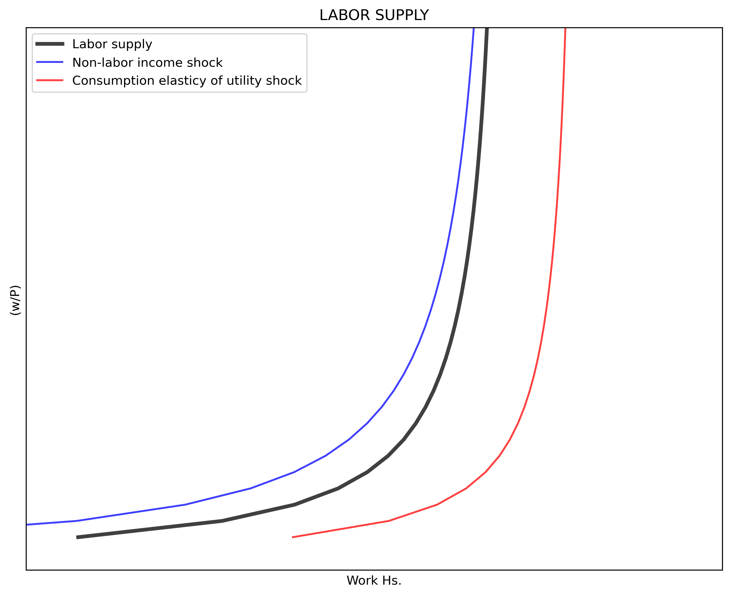
Labor supply $N^S$ is the number of hours not spent in leisure. Note that $N^S$ decreases with $I$ and increases with $(w/P)$.
$$ \begin{align} N^S &= T - L^* \\[10pt] N^S &= T - (1-\beta) \left[\frac{I + T (w/P)}{(w/P)} \right] \end{align} $$
If $I=0$, then labor supply does not depend on $w/P \to N^S = \beta T$.
The following code shows labor supply (in black) and shocks to non-labor income $\Delta I = 25$ (in blue) and to consumption elasticity of utility $\Delta \beta = 0.10$ (in red). Note that in this construction $N^S$ does not bend-backwards as is typically shows in economic textbooks.
#%% *** CELL 3 ***
"============================================================================"
"9|LABOR SUPPLY"
def Nsupply(rW, beta, I):
    Lsupply = T - (1-beta)*((T*rW + I)/rW)
    return Lsupply

D_I = 25     # Shock to non-income labor
D_b = 0.10   # Shock to beta

Ns   = Nsupply(rW, beta    , I)
Ns_b = Nsupply(rW, beta+D_b, I)
Ns_I = Nsupply(rW, beta    , I+D_I)


"============================================================================"
"10|PLOT LABOR SUPPLY"
# AXIS RANGE
y_max = np.max(Ns)
axis_range = [0, T, 0, y_max]

# BUILD PLOT
fig, ax = plt.subplots(figsize=(10, 8), dpi=dpi)
ax.set(title="LABOR SUPPLY", xlabel="Work Hs.", ylabel=r'(w/P)')
# ADD LABOR SUPPLY LINES
ax.plot(Ns  , rW, "k", alpha=0.75, label="Labor supply", linewidth=3)
ax.plot(Ns_I, rW, "b", alpha=0.75, label="Non-labor income shock")
ax.plot(Ns_b, rW, "r", alpha=0.75, label="Consumption elasticy of utility shock")
ax.yaxis.set_major_locator(plt.NullLocator())      # Hide ticks
ax.xaxis.set_major_locator(plt.NullLocator())      # Hide ticks
# SETTINGS
ax.grid()
ax.legend()
plt.axis(axis_range)
plt.show()
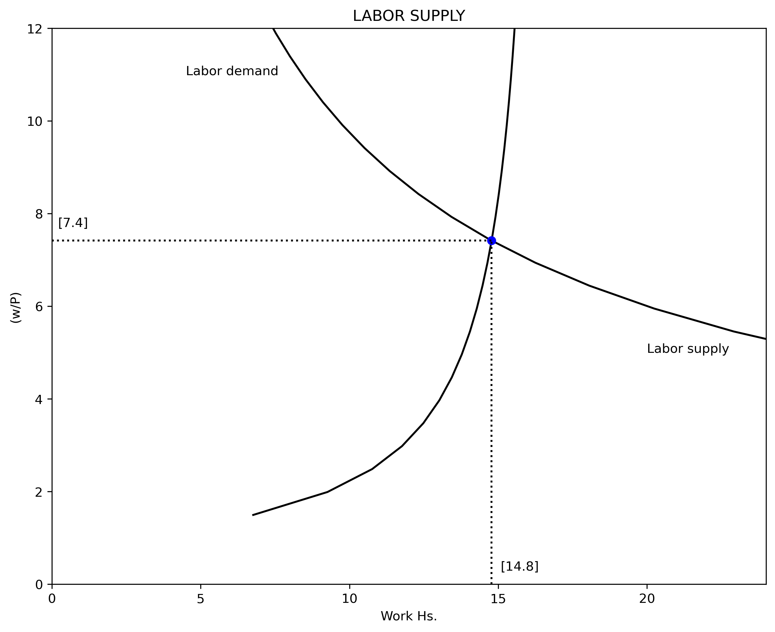
Equilibrium
We can now calculate the equilibrium condition: the value of $(w/P)_0$ which makes $N^D\left(\left(\frac{w}{P}\right)_0\right) = N^S\left(\left(\frac{w}{P}\right)_0\right)$. We can define a new function $\Theta$ equal to zero at $\left(\frac{w}{P}\right)_0$:
$$ \begin{align} \Theta \left[\left(\frac{w}{P}\right)_0 \right] &= 0 = N^D \left[\left(\frac{w}{P} \right)_0 \right] - N^S \left[\left(\frac{w}{P}\right)_0 \right] \\[10pt] \Theta \left[\left(\frac{w}{P}\right)_0 \right] &= 0 = \left[K \cdot \left[\frac{(1-\alpha)A}{(w/P)}\right]^{1/\alpha} \right] - \left[T(1-\beta) \left[\frac{I + T(w/P)}{(w/P)} \right] \right] \end{align} $$
Our model does not have linear equations that would allow for an easy algebraic solution. We can use Python to calculate the value (root) of $\left( \frac{w}{P} \right)$ that makes $\Theta = 0$. For this we need the “root” function from the SciPy library.
#%% *** CELL 4 ***
"============================================================================"
"11|OPTIMIZATION PROBLEM: FIND EQUILIBRIUM VALUES"
def Eq_Wage(rW):
    Eq_Wage = Ndemand(A, K, rW, alpha) - Nsupply(rW, beta, I)
    return Eq_Wage

rW_0 = 10                             # Initial value (guess)
rW_star = root(Eq_Wage, rW_0)         # Equilibrium: Wage
N_star  = Nsupply(rW_star.x, beta, I) # Equilibrium: Labor


"============================================================================"
"12|PLOT LABOR MARKET EQUILIBRIUM"
#AXIS RANGE
y_max = rW_star.x*2
axis_range = [0, T, 0, 12] # Set the axes range

# BUILD PLOT
fig, ax = plt.subplots(figsize=(10, 8), dpi=dpi)
ax.set(title="LABOR SUPPLY", xlabel="Work Hs.", ylabel=r'(w/P)')
# ADD LABOR DEMAND AND SUPPLY
ax.plot(Ns[1:T], rW[1:T], "k", label="Labor supply")
ax.plot(Nd[1:T], rW[1:T], "k", label="Labor demand")
plt.plot(N_star, rW_star.x, 'bo')
plt.axvline(x=N_star   , ymin=0, ymax=rW_star.x/12, ls=':', color='k')
plt.axhline(y=rW_star.x, xmin=0, xmax=N_star/T    , ls=':', color='k')
# ADD LABELS
plt.text( 4.5      , 11, "Labor demand")
plt.text(20        ,  5, "Labor supply")
plt.text(0.2       , rW_star.x+0.3, np.round(rW_star.x, 1))
plt.text(N_star+0.3, 0.3          , np.round(N_star, 1))
# SETTINGS
plt.axis(axis_range)
plt.show()