Endogenous Growth with R&D
Introduction
A well-known result of the Solow Model is that growth remains as an exogenous explanation. That is, it goes unexplained by the model. Growth (in the long-run) does not depend on the savings rate, but on the growth rate of technology ($A$). The growth rate of $A$ is an assumption given to the model. Yet, Solow Model is useful because it provides a number of important insights.
Endogenous growth models produce an endogenous growth rate. One way to endogenize growth is by adding to the model a production function of technology. In this sense, the R&D growth model can be interpreted as an extension of Solow model.
The R&D Growth model
The R&D model assumes two sectors: (1) production of goods and (2) production of new ideas (technology). Factors of production, capital $(K)$ and labor $(L)$, are split between these two sectors. The model is built in continuous time. Labor grows at constant rate $n$.
Production of goods
Assume the following Cobb-Douglas function with constant returns to scale and labor-augmenting technology.
$$ \begin{equation} Y(t) = \left[(1-a_K)K \right]^{\alpha} \left[A(t) (1-a_L) L(t) \right]^{1-\alpha}; \quad a, \alpha \in (0, 1) \end{equation} $$
where $a_K$ and $a_L$ represent the share of capital and labor allocated to the production of new ideas. Therefore, $(1-a_K)$ and $(1-a_L)$ represent the share of capital and labor allocated to the production of new goods.
Accumulation of new capital
Similar to Solow model, the accumulation of new capital depends on an exogenous fixed savings rate $(s)$ of output. For simplicity, assume there is no depreciation.
$$ \begin{equation} \dot{K}(t) = sY(t) \end{equation} $$
Production of new ideas
The production of new ideas follows a Cobb-Douglas function that may or may not have constant returns to scale. Whether the returns to scale in the production of new ideas is decreasing, constant, or increasing depends on the assumption of how factors of production interact in the R&D industry. Because this industry produces ideas, the argument of “replication” (if you double inputs you double output) does not have to hold as in the case of physical output.
$$ \begin{equation} \dot{A}(t) = B \left[a_K K(t) \right]^{\beta} \left[a_l L(t) \right]^{\gamma} A(t)^{\theta}; \quad B>0, \beta\geq 0, \gamma\geq 0 \end{equation} $$
The dot on top of $A$ denotes (instantaneous) change of technology and $B$ is a shift parameters. The exponent $\theta$ captures how the accumulated knowledge affects the discovery of new ideas.
If the more knowledge already discovered makes it more difficulty to discover new ideas, then $\theta$ is negative. If the accumulated knowledge makes it easier to discover new ideas, then $\theta$ is larger than one.
Solving the model
Solving the model implies finding how the growth rates look in the steady-state. Are growth rates constant? Or do they change with time?
Let $g_K(t)$ and $g_A(t)$ denote the growth rates of capital and technology. Then, we want to study the conditions in which $\dot{g}_K(t)=\dot{g}_A(t)=0$. To do this, we need to calculate the growth rates, and then set them constant (set the change in the growth rate equal to zero).
The steady-state of capital
We can proceed in three steps to find the steady-state of capital. First, input the production function (of goods) into the motion function of capital. Second, calculate the growth rate of capital. Third, set the change in the growth equal to zero and “solve for” growth of capital in terms of growth of technology. The last step will be useful to plot the dynamics of the model.
The growth rates of capital and technology are $g_K(t) \equiv \frac{\dot{K}(t)}{K(t)}$ and $g_A(t) \equiv \frac{\dot{A}(t)}{A(t)}$.
$$ \begin{align} \dot{K}(t) &= s (1-a_K)^{\alpha} (1-a_L)^{1-\alpha} \cdot K(t)^{\alpha} A(t)^{1-\alpha} L(t)^{1-\alpha} \\[10 pt] g_K(t) &= s (1-a_K)^{\alpha} (1-a_L)^{1-\alpha} \left[\frac{A(t)L(t)}{K(t)} \right]^{1-\alpha} \\[10 pt] \frac{\dot{g}_K(t)}{g_K(t)} &= (1-\alpha) \left[g_A(t) + n - g_K(t) \right] \end{align} $$
$K$ will grow if $\left[g_A(t) + n - g_K(t) \right] > 0$. Now set $g_K(t) = 0$ and “solve for” $g_K(t)$ in terms of $g_A(t)$.
$$ \begin{equation} g_K(t) = n + g_A(t) \end{equation} $$
The last line is a simple linear equation with intercept $n$ and slope 1 in terms of $g_A(t)$. Also, note that $g_K(t)$ does not depend on the savings rate or the other parameters of the production function (of final goods). Similar to Solow model, the growth rate of $K$ equals (in the steady state) the growth rate of population plus the growth rate of technology.
The steady-state of technology
We can proceed in a similar way to find the steady-state of technology. First, find the growth rate of technology. Then, set the change in the growth rate of technology equal to zero, and then solve for $g_K(t)$ in terms of $g_A(t)$.
$$ \begin{align} \dot{A}(t) &= B \left[a_K K(t) \right]^{\beta} \left[a_l L(t) \right]^{\gamma} A(t)^{\theta} \\[10pt] g_A(t) &= B \left[a_K K(t) \right]^{\beta} \left[a_L L(t) \right]^{\gamma} A(t)^{\theta - 1} \\[10pt] \frac{\dot{g}_A(t)}{g_A(t)} &= \beta g_K(t) + \gamma n + (\theta - 1) g_A(t) \end{align} $$
$A$ will grow if $\left[\beta g_K(t) + \gamma n + (\theta - 1) g_A(t) \right] > 0$. Now, assuming $g_A(t) = 0$:
$$ \begin{equation} g_K(t) = -\frac{\gamma n}{\beta} + \frac{(1-\theta)}{\beta} g_A(t) \end{equation} $$
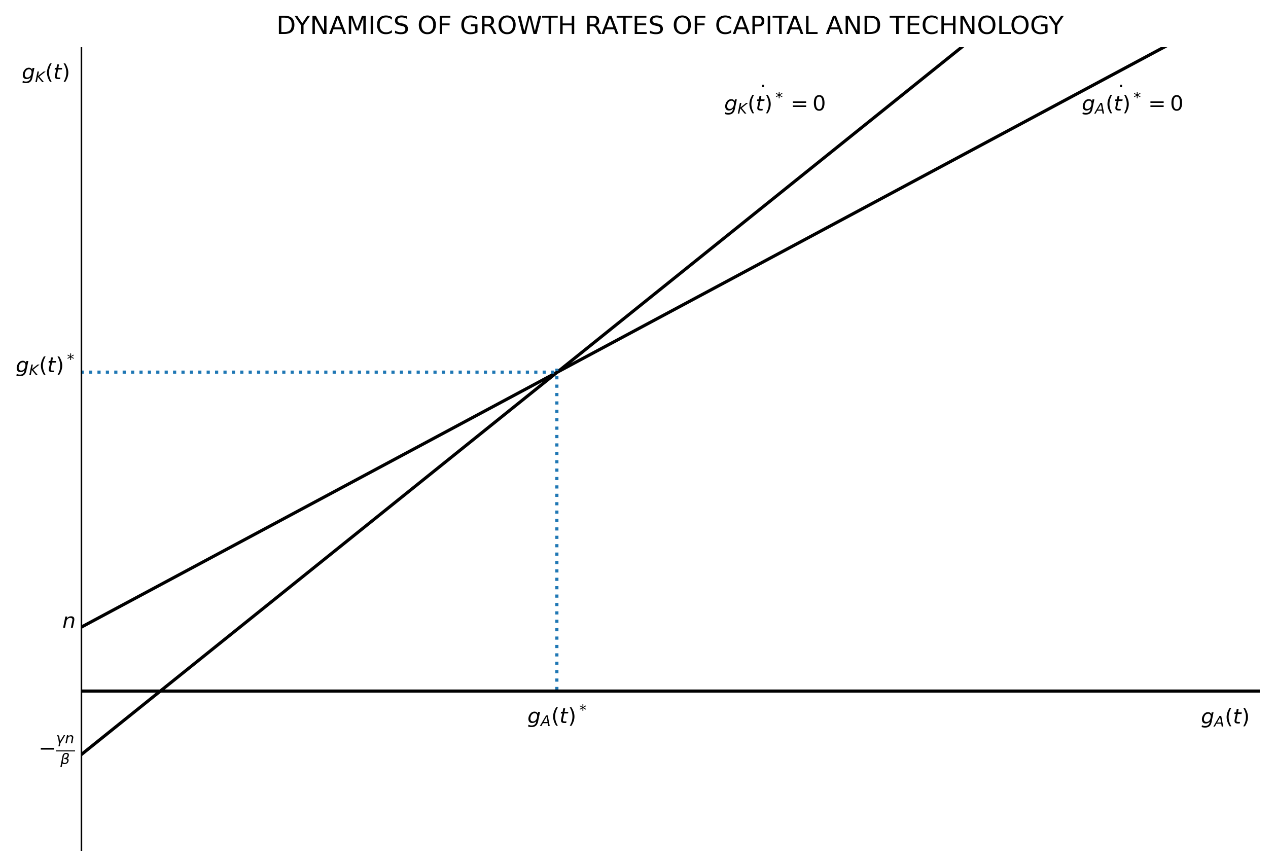
The last line also is a simple linear equation, with intercept $-\frac{\gamma n}{\beta}$ and slope $\frac{(1-\theta)}{\beta}$ with respect to $g_A(t)$. The slope is positive if $1-\theta>0$, and the model has in equilibrium if $\frac{(1-\theta)}{\beta}>1$ (see the figure below).
The steady-state
The R&D model has two equations with two unknowns.
$$ \begin{align} g_K(t) &= n + g_A(t) \\[10pt] g_K(t) &= -\frac{\gamma n}{\beta} + \frac{(1-\theta)}{\beta} g_A(t) \end{align} $$
Solving this system of equation yields the (constant) growth rates in the steady-state.
$$ \begin{align} g_K(t)^* &= n \frac{\beta + \gamma}{1-(\theta + \gamma)} + n \\[5 pt] g_A(t)^* &= n \frac{\beta + \gamma}{1-(\theta + \gamma)} \end{align} $$
Consider the following:
- Note that $g_K(t)^* > g_A(t)^*$
- If $n = 0$, then $g_K(t)^* = g_A(t)^* = 0$
- Savings rate $(s)$ does not affect long-run growth rates
- Neither $a_L$ or $a_K$ affect long-run growth rates
To be more precise, this model can be considered a semi-endogenous growth model. Long-run growth rates depends on endogenous variables of the model, but also on the exogenous growth rate of population.
The Python code
We can now plot both saddle-paths $(\dot{g}_A(t)=0, \dot{g}_K(t)=0)$ using Python. These are two linear equations.
#%% *** CELL 1 ***
"|***************************************************************************|"
"1|IMPORT PACKAGES"
import numpy as np               # Package for scientific computing with Python
import matplotlib.pyplot as plt  # Matplotlib is a 2D plotting library


"|***************************************************************************|"
"2|DEFINE PARAMETERS AND ARRAYS"
# Code parameters
dpi = 300
step  = 0.01
# Model parameters
n     = 0.02      # Growth rate of population
beta  = 0.50      # Exponent of capital in the production of ideas
gamma = 1 - beta  # Exponent of labor in the priduction of ideas
theta = 0.25      # Exponent of technology in the production of ideas

# Arrays
gA = np.arange(0, 1, step) # Array between 0 and 1 with step size=0.01
gK = n + gA


"|***************************************************************************|"
"3|DEFINE AND POPULATE THE SADDLE-PATH FUNCTIONS"
# Saddle paths for K and A
ss_K = n + gA
ss_A = -(gamma*n)/beta + (1 - theta)/beta*gA

# Intercept of K saddle-path
ss_int = -(gamma*n)/beta


"|***************************************************************************|"
"4|EQUILIBRIUM VALUES"
A_star = n*(beta + gamma)/(1 - (theta + gamma))
K_star = n + A_star


"|***************************************************************************|"
"5|PLOT THE SADDLE-PATH"
### AXIS RANGE
axis_range = [0, gA.max()*0.2, -0.05, gK.max()*0.2]

### BUILD FIGURE
plt.figure(figsize=(10, 7), dpi=dpi)
plt.title("DYNAMICS OF GROWTH RATES OF CAPITAL AND TECHNOLOGY")
plt.plot(gA, ss_A, "k-", label=r'$g_A(t)$')
plt.plot(gA, ss_K, "k-", label=r'$g_K(t)$')
### EQUILIBRIUM MARKS
plt.axvline(A_star, -axis_range[2]/(0.25), (0.05+K_star)/0.25  , ls=":")
plt.axhline(K_star, 0.0                  , A_star/axis_range[1], ls=":")
### AXIS
plt.axvline(0, color="k")                    # Add vertical axis
plt.axhline(0, color="k")                    # Add horizontal axis
plt.xticks([], [])                           # Hide x-axis ticks
plt.yticks([], [])                           # Hide y-axis ticks
plt.text(-0.01             , axis_range[3]-0.01, r'$g_K(t)$')  # x-axis label
plt.text(axis_range[1]-0.01, -0.01             , r'$g_A(t)$')  # y-axis label
### VALUES AND LABELS
plt.text(axis_range[1]-0.03, axis_range[3]-0.02, r'$\dot{g_A(t)^*}=0$')
plt.text(axis_range[1]-0.09, axis_range[3]-0.02, r'$\dot{g_K(t)^*}=0$')
plt.text(A_star, -0.01 , r'$g_A(t)^*$', horizontalalignment="center")
plt.text(-0.001, K_star, r'$g_K(t)^*$', horizontalalignment="right")
plt.text(-0.001, n     , r'$n$'       , horizontalalignment="right")
plt.text(-0.001, ss_int, r'$-\frac{\gamma n}{\beta}$',
         horizontalalignment="right")
### SETINGS
plt.box(False)
plt.axis(axis_range)
plt.show()
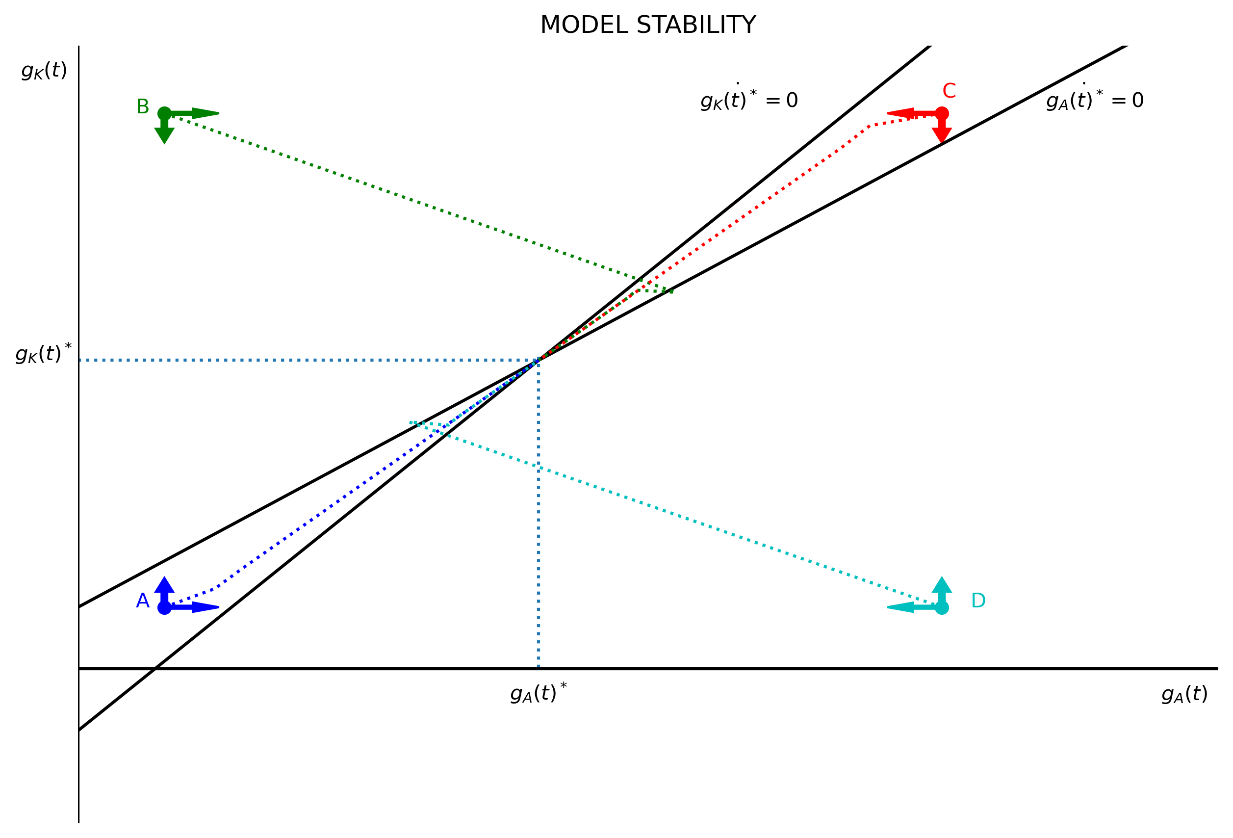
Model stability
This is a stable model. Any starting point outside the steady-state will return to equilibrium. The code below follows the model dynamics for $A$ and $K$:
$$ \begin{align} g_A(t+1) &= g_K(t) + \dot{g}_K(t) \\[10pt] g_K(t+1) &= g_A(t) + \dot{g}_A(t) \\[10pt] g_A(t+1) &= g_K(t) + (1-\alpha) \left[g_A(t) + n - g_K(t) \right] \\[10pt] g_K(t+1) &= g_A(t) + \beta g_K(t) + \gamma n + (\theta - 1)g_A(t) \end{align} $$
Now set four arbitrary starting points: A (blue), B (green), C (red), D (cyan). These starting points will be located in the four quadrants of the model dynamics plot. From these four stating points, the code performs 75 iterations. The plot shows that the dynamics of starting points A and C remain between the two saddle paths, while starting points B and D cross over a saddle path to then approach the steady-state.
#%% *** CELL 2 ***
"|***************************************************************************|"
"6|DEFINE PARAMETERS AND ARRAYS"
# Parameters
alpha = 0.60  # Exponent of capital in the production of goods


"|***************************************************************************|"
"7|STABILITY DYNAMICS"
iterations = 75

" | Starting Poin A (blue)"
# Create arrays to store model dynamics
A_gA = np.zeros(iterations)
A_gK = np.zeros(iterations)
# Set arbitrary initial values
A_gA[0] = 0.015
A_gK[0] = 0.020

for j in range(1, iterations):
    A_gA[j] = A_gA[j-1] + beta*A_gK[j-1] + gamma*n + (theta-1)*A_gA[j-1]
    A_gK[j] = A_gK[j-1] + (1-alpha)*(A_gA[j-1] + n - A_gK[j-1])

" | Starting Poin B (green)"
# Create arrays to store model dynamics
B_gA = np.zeros(iterations)
B_gK = np.zeros(iterations)
# Set arbitrary initial values
B_gA[0] = 0.015
B_gK[0] = 0.180

for j in range(1, iterations):
    B_gA[j] = B_gA[j-1] + beta*B_gK[j-1] + gamma*n + (theta-1)*B_gA[j-1]
    B_gK[j] = B_gK[j-1] + (1-alpha)*(B_gA[j-1] + n - B_gK[j-1])

" | Starting Poin C (red)"
# Create arrays to store model dynamics
C_gA = np.zeros(iterations)
C_gK = np.zeros(iterations)
# Set arbitrary initial values
C_gA[0] = 0.150
C_gK[0] = 0.180

for j in range(1, iterations):
    C_gA[j] = C_gA[j-1] + beta*C_gK[j-1] + gamma*n + (theta-1)*C_gA[j-1]
    C_gK[j] = C_gK[j-1] + (1-alpha)*(C_gA[j-1] + n - C_gK[j-1])

" | Starting Poin D (cyan)"
# Create arrays to store model dynamics
D_gA = np.zeros(iterations)
D_gK = np.zeros(iterations)
# Set arbitrary initial values
D_gA[0] = 0.150
D_gK[0] = 0.020

for j in range(1, iterations):
    D_gA[j] = D_gA[j-1] + beta*D_gK[j-1] + gamma*n + (theta-1)*D_gA[j-1]
    D_gK[j] = D_gK[j-1] + (1-alpha)*(D_gA[j-1] + n - D_gK[j-1])


"|***************************************************************************|"
"8|PLOT THE SADDLE-PATH"
### AXIS RANGE
axis_range = [0, gA.max()*0.2, -0.05, gK.max()*0.2]

# BUILD PLOT
plt.figure(figsize=(10, 7), dpi=dpi)
plt.title("MODEL STABILITY")
plt.plot(gA, ss_A, "k-", label=r'$g_A(t)$')
plt.plot(gA, ss_K, "k-", label=r'$g_K(t)$')
### EQUILIBRIUM MARKS
plt.axvline(A_star, -axis_range[2]/(0.25), (0.05+K_star)/0.25  , ls=":")
plt.axhline(K_star, 0.0                  , A_star/axis_range[1], ls=":")
### AXIS
plt.axvline(0, color="k")  # Add vertical axis
plt.axhline(0, color="k")  # Add horizontal axis
plt.xticks([], [])         # Hide x-axis ticks
plt.yticks([], [])        # Hide y-axis ticks
plt.text(-0.01              , axis_range[3]-0.01, r'$g_K(t)$')  # x-axis label
plt.text(axis_range[1]-0.01, -0.01              , r'$g_A(t)$')  # y-axis label
### VALUES AND LABELS
plt.text(A_star, -0.01 , r'$g_A(t)^*$', horizontalalignment="center")
plt.text(-0.001, K_star, r'$g_K(t)^*$', horizontalalignment="right")
plt.text(axis_range[1]-0.03, axis_range[3]-0.02, r'$\dot{g_A(t)^*}=0$')
plt.text(axis_range[1]-0.09, axis_range[3]-0.02, r'$\dot{g_K(t)^*}=0$')
### MODEL DYNAMICS
plt.plot(A_gA[0], A_gK[0], "bo")
plt.plot(A_gA   , A_gK   , "b:")
plt.plot(B_gA[0], B_gK[0], "go")
plt.plot(B_gA   , B_gK   , "g:")
plt.plot(C_gA[0], C_gK[0], "ro")
plt.plot(C_gA   , C_gK   , "r:")
plt.plot(D_gA[0], D_gK[0], "co")
plt.plot(D_gA   , D_gK   , "c:")
plt.text(A_gA[0]-0.005, A_gK[0]      , "A", color="b")
plt.text(B_gA[0]-0.005, B_gK[0]      , "B", color="g")
plt.text(C_gA[0]      , C_gK[0]+0.005, "C", color="r")
plt.text(D_gA[0]+0.005, D_gK[0]      , "D", color="c")
# ARROWS
plt.arrow(A_gA[0], A_gK[0],  0.005, 0    , color="b")
plt.arrow(A_gA[0], A_gK[0],  0    , 0.005, color="b")
plt.arrow(B_gA[0], B_gK[0],  0.005, 0    , color="g")
plt.arrow(B_gA[0], B_gK[0],  0    ,-0.005, color="g")
plt.arrow(C_gA[0], C_gK[0], -0.005, 0    , color="r")
plt.arrow(C_gA[0], C_gK[0],  0    ,-0.005, color="r")
plt.arrow(D_gA[0], D_gK[0], -0.005, 0    , color="c")
plt.arrow(D_gA[0], D_gK[0],  0    , 0.005, color="c")
### SETTINGS
plt.box(False)
plt.axis(axis_range)
plt.show()