The IS-LM Model
Introduction
The IS-LM (or Hicks-Hansen) model shows the combinations of interest rate (vertical axis) and income (horizontal axis) for which the goods market (IS) and the loan market (LM) are in equilibrium. There is one particular combination of interest rate and income that is consistent with equilibrium in both markets simultaneously.
In the graphic version of the model, all the points in the IS schedule represent equilibrium in the goods market. Similarly, all the points in the LM schedule represents equilibrium in the loanable funds market.
This model treats the price level as exogenous (given and fixed). In this sense, the IS-LM model is applicable in the context of substantia idle resources, when changes in income have no effect on the price level.
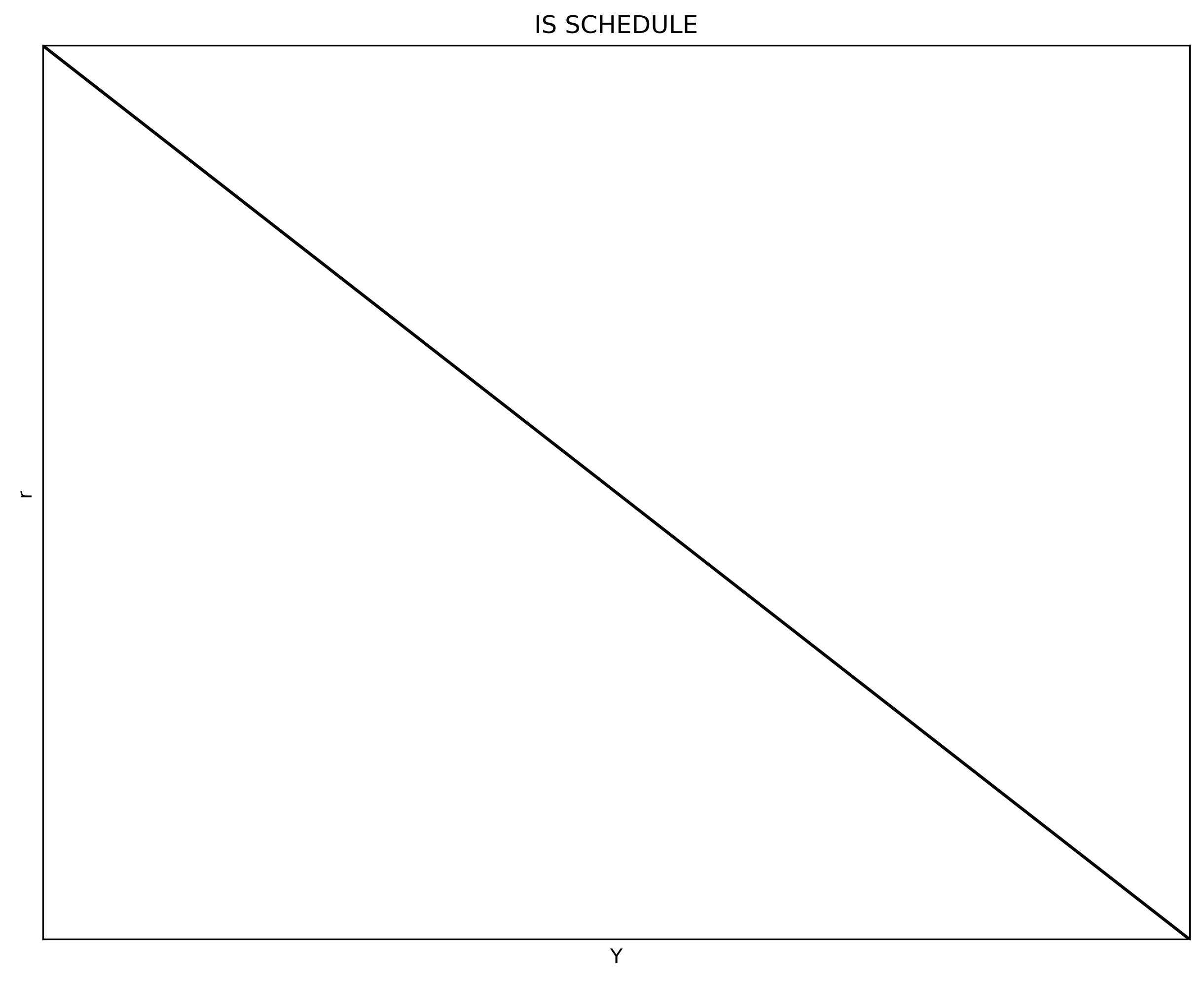
The IS schedule (Investment-Saving)
The IS schedule is derived from the equilibrium condition where output
where
Assume that
where
Assume now a simple linear relationship between investment and the interest rate
where
We can also assume that imports follow a similar functional form than household’s domestic consumption:
where
To derive the IS schedule we need to use the consumption, investment, and import functions and solve for
Note that the larger
The following code plots the IS schedule using the above information. The first part of the code imports the required Python packages. The second part of the code defines the parameters and arrays. The third part of the code defines and populates the IS schedule. The fourth part of the code plots the IS schedule.
#%% *** CELL 1 ***
"============================================================================"
"1|IMPORT PACKAGES"
import numpy             as np   # Package for scientific computing
import matplotlib.pyplot as plt  # Matplotlib is a 2D plotting library


"============================================================================"
"2|DEFINE PARAMETERS AND ARRAYS"
# Code parameters
dpi = 300
# IS parameters
Y_size = 100
a      =  20    # Autonomous consumption
b      =   0.2  # Marginal propensity to consume
alpha  =   5    # Autonomous imports
beta   =   0.2  # Marginal propensity to import
T      =   1    # Taxes
I      =  10    # Investment intercept (when i = 0)
G      =   8    # Government spending
X      =   2    # Exports (given)
d      =   5    # Investment slope wrt to i
# Arrays
Y = np.linspace(0, Y_size, Y_size*2)  # Array values of Y


"============================================================================"
"3|DEFINE AND POPULATE THE IS-SCHEDULE"
def i_IS(a, alpha, b, beta, T, I, G, X, d, Y):
    i_IS = ((a-alpha)-(b-beta)*T + I + G + X - (1-b+beta)*Y)/d
    return i_IS

def Y_IS(a, alpha, b, beta, T, I, G, X, d, i):
    Y_IS = ((a-alpha)-(b-beta)*T + I + G + X - d*i)/(1-b+beta)
    return Y_IS

i = i_IS(a, alpha, b, beta, T, I, G, X, d, Y)


"============================================================================"
"4|PLOT THE IS-SCHEDULE"
### AXIS RANGE
y_max = np.max(i)
x_max = Y_IS(a, alpha, b, beta, T, I, G, X, d, 0)
axis_range = [0, x_max, 0, y_max]

### BUILD PLOT
fig, ax = plt.subplots(figsize=(10, 8), dpi=dpi)
ax.set(title="IS SCHEDULE", xlabel=r'Y', ylabel=r'r')
ax.plot(Y, i, "k-")
### AXIS
ax.yaxis.set_major_locator(plt.NullLocator())   # Hide ticks
ax.xaxis.set_major_locator(plt.NullLocator())   # Hide ticks
### SETTINGS
plt.axis(axis_range)
plt.show()
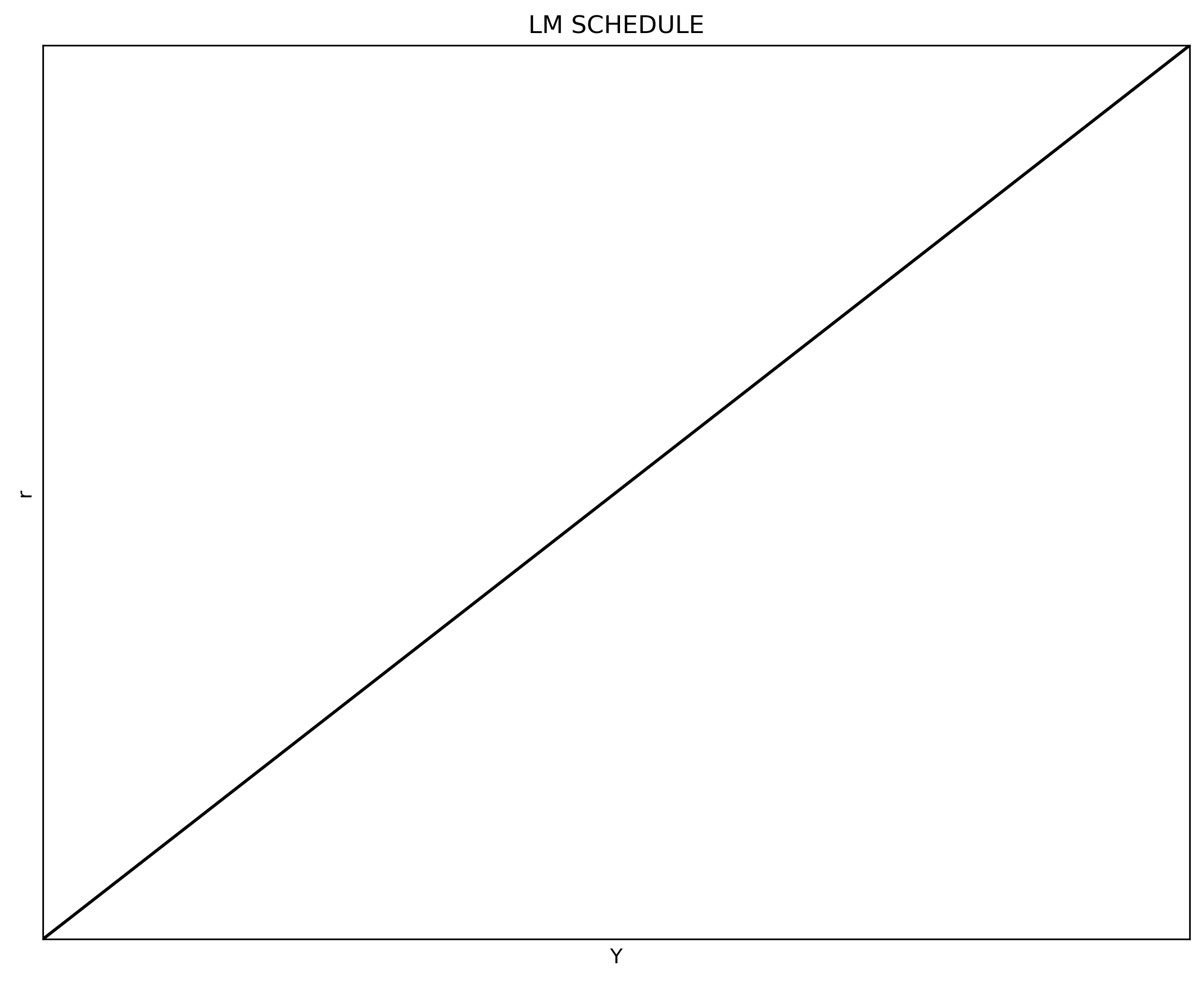
The LM schedule (Liquidity preference-Money supply)
To build the LM schedule we need money supply
- precautionary reasons (e.g. save for a rainy-day), (2)
- to perform transaction
- speculation reasons.
Expressing
Where each term represent precautionary, transaction, and speculation reasons to demand money respectively. Note that the amount of money needed for transactions depends on the level of income. The interest rate has a negative relationship with money demand due to Keynes' expectations theory (not covered here).
Since in equilibrium
Note that if the interest rate has no effect on money demand
We can plot the LM schedule in a similar way we did for the IS schedule.
#%% *** CELL 2 ***
"============================================================================"
"5|DEFINE PARAMETERS"
# LM Parameters
c1 = 1000       # Precautionary money demand
c2 = 10         # Transaction money demand
c3 = 10         # Speculation money demand
Ms = 20000      # Nominal money supply
P  = 20         # Price level


"============================================================================"
"6|DEFINE AND POPULATE THE LM-SCHEDULE"
def i_LM(c1, c2, c3, Ms, P, Y):
    i_LM = (c1 - Ms/P)/c3 + c2/c3*Y
    return i_LM

i = i_LM(c1, c2, c3, Ms, P, Y)


"============================================================================"
"7|PLOT THE LM-SCHEDULE"
### AXIS RANGE
y_max = np.max(i)
axis_range = [0, Y_size, 0, y_max]

### BUILD PLOT
fig, ax = plt.subplots(figsize=(10, 8), dpi=dpi)
ax.set(title="LM SCHEDULE", xlabel=r'Y', ylabel=r'r')
ax.plot(Y, i, "k-")
ax.yaxis.set_major_locator(plt.NullLocator())   # Hide ticks
ax.xaxis.set_major_locator(plt.NullLocator())   # Hide ticks
### SETTINGS
plt.axis(axis_range)
plt.show()
Equilibrium
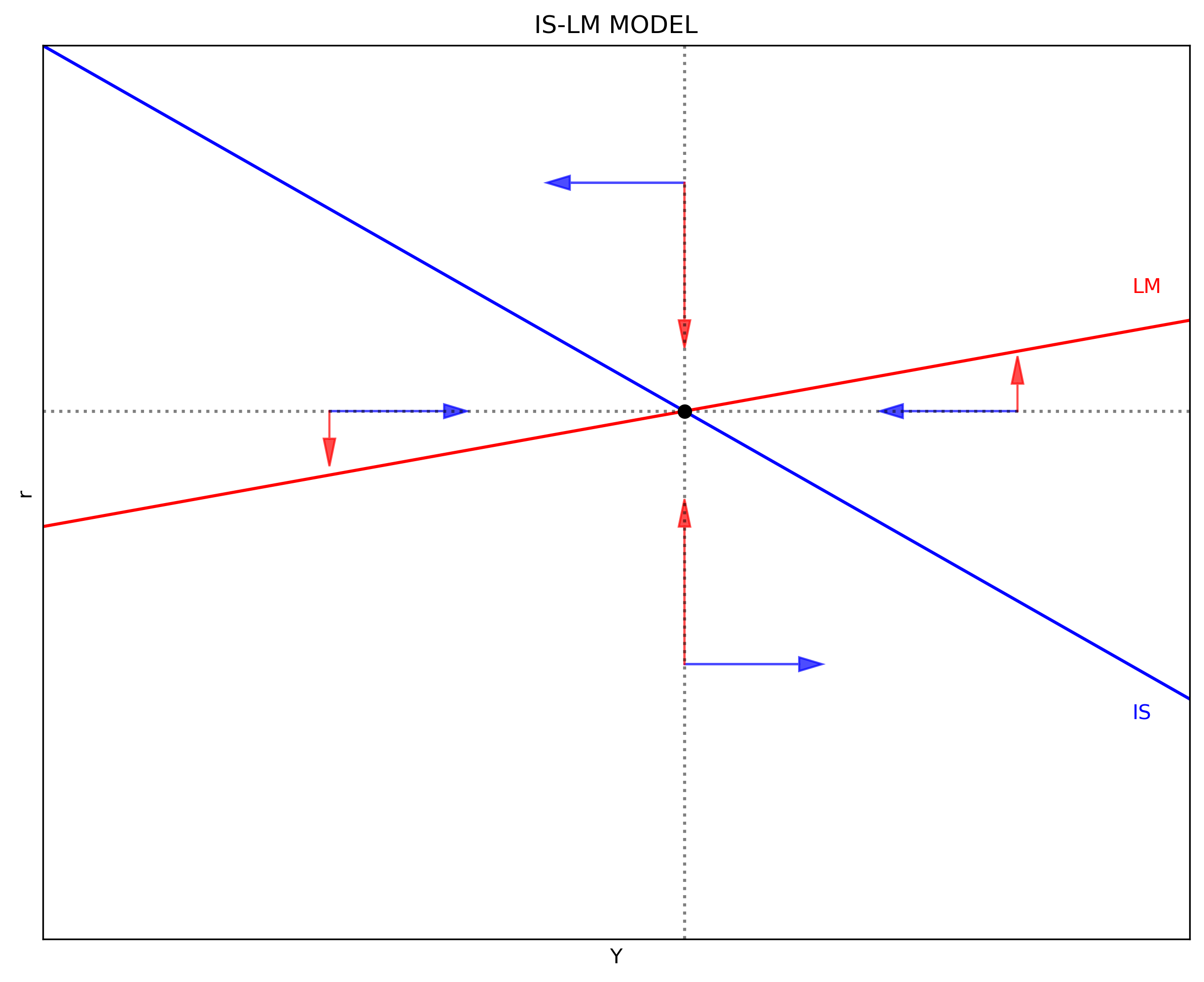
Note that the LM and IS do not share any variable. This means that any shock shifts only one of the schedules. This construction conveniently separates monetary policy as shifts of the LM schedule from fiscal policy as shifts of the IS schedule.
There is a pair $(Y^, i^)
And the interest rate of equilibrium would be:
The next code plots the IS-LM model and locates four arrows showing the dynamics of the model when the economy is out of equilibrium. The IS and LM schedules and their dynamics are denoted in blue and red respectively.
#%% *** CELL 3 ***
"============================================================================"
"8|DEFINE NEW PARAMETERS"
# IS new parameters
a = 100              # Autonomous consumption
b = 0.2              # Marginal propensity to consume
alpha = 5            # Autonomous imports
beta  = 0.15         # Marginal propensity to import
T = 1                # Taxes
I = 10               # Investment intercept (when i = 0)
G = 20               # Government spending
X = 5                # Exports (given)
d = 2                # Investment slope wrt to i
# LM new parameters
c1 = 2500            # Precautionary money demand
c2 = 0.75            # Transaction money demand
c3 = 5               # Speculation money demand
Ms = 23500           # Nominal money supply
P  = 10              # Price level


"============================================================================"
"9|CALCULATE EQUILIBRUM VALUES"

iIS = i_IS(a, alpha, b, beta, T, I, G, X, d, Y)
iLM = i_LM(c1, c2, c3, Ms, P, Y)

Y_star1 = ((a-alpha) - (b-beta)*T + I + G + X)/d
Y_star2 = (1/c3) * (c1 - Ms/P)
Y_star3 = (1 - b + beta)/d + (c2/c3)
Y_star  = (Y_star1 - Y_star2)/Y_star3

i_star1 = (1/c3)*(c1 - Ms/P)
i_star2 = (c2/c3)*Y_star
i_star  = i_star1 + i_star2


"============================================================================"
"10|PLOT THE IS-LM model"
### AXIS RANGE
y_max = np.max(iIS)
axis_range = [0, Y_size, 0, y_max]

### BUILD PLOT
fig, ax = plt.subplots(figsize=(10, 8), dpi=dpi)
ax.set(title="IS-LM MODEL", xlabel=r'Y', ylabel=r'r')
ax.plot(Y, iIS, "b-")
ax.plot(Y, iLM, "r-")
### AXIS
ax.yaxis.set_major_locator(plt.NullLocator())  # Hide ticks
ax.xaxis.set_major_locator(plt.NullLocator())  # Hide ticks
### ARROWS AND EQUILIBRIUM POINT
ax.arrow(25, i_star, 10,  0, head_length=2, head_width=1, color='b', alpha=0.7)
ax.arrow(25, i_star,  0, -2, head_length=2, head_width=1, color='r', alpha=0.7)
ax.arrow(Y_star, 20, 10,  0, head_length=2, head_width=1, color='b', alpha=0.7)
ax.arrow(Y_star, 20,  0, 10, head_length=2, head_width=1, color='r', alpha=0.7)
ax.arrow(85, i_star,-10,  0, head_length=2, head_width=1, color='b', alpha=0.7)
ax.arrow(85, i_star,  0,  2, head_length=2, head_width=1, color='r', alpha=0.7)
ax.arrow(Y_star, 55,-10,  0, head_length=2, head_width=1, color='b', alpha=0.7)
ax.arrow(Y_star, 55,  0,-10, head_length=2, head_width=1, color='r', alpha=0.7)
plt.plot(Y_star, i_star, 'ko')                      # Equilibrium point
plt.axvline(x=Y_star, ls=':', color='k', alpha=0.5) # Equilibrium line
plt.axhline(y=i_star, ls=':', color='k', alpha=0.5) # Equilibrium line
### LABELS
plt.text(95, 16, "IS", color='b')
plt.text(95, 47, "LM", color='r')
### SETTINGS
plt.axis(axis_range)
plt.show()
Dynamics
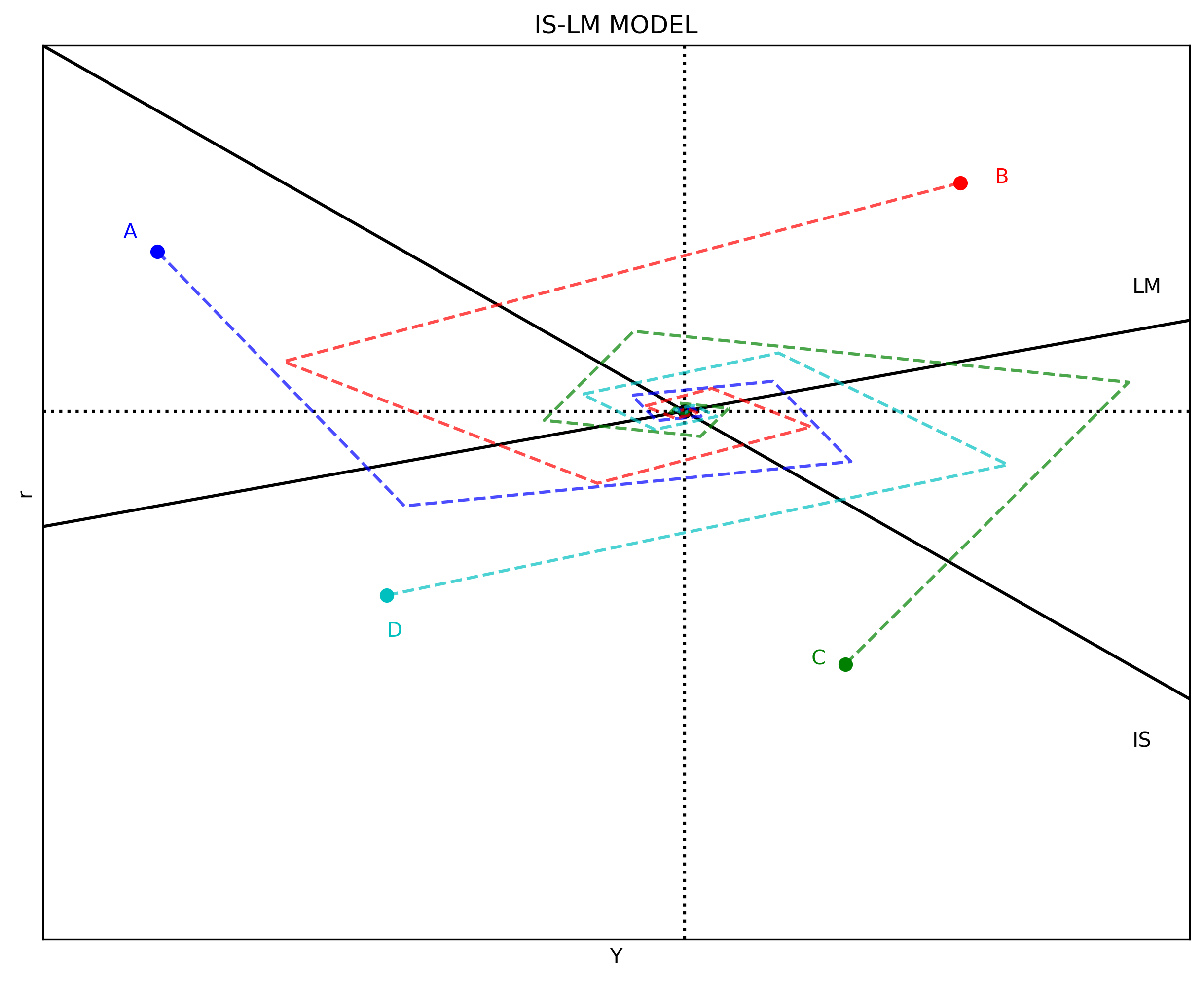
The arrows in the above figure shows that the model is stable. The economy always converge back to equilibrium. The code below shows the dynamics towards equilibrium starting from four disequilibrium points: A in blue, B in red, C in green, and D in olive. For the illustration purposes of this example, ten iterations starting from each point is enough to show the dynamics towards equilibrium.
Horizontal changes
#%% *** CELL 4 ***
"============================================================================"
"11|CALCULATE THE DYNAMICS FOR DISEQUILIBRIUM POINTS"
iterations= 10

" |STARTING POINT A"
YA, iA = 10, 50   # Initial values

A_i_LM = np.zeros(iterations)
A_Y_IS = np.zeros(iterations)

A_Y_IS[0] = YA
A_i_LM[0] = iA

for j in range(1, iterations):
    A_Y_IS[j] = Y_IS(a, alpha, b, beta, T, I, G, X, d, A_i_LM[j-1])
    A_i_LM[j] = i_LM(c1, c2, c3, Ms, P, A_Y_IS[j-1])

" |STARTING POINT B"
YB, iB = 80, 55   # Initial values

B_i_LM = np.zeros(iterations)
B_Y_IS = np.zeros(iterations)

B_Y_IS[0] = YB
B_i_LM[0] = iB

for j in range(1, iterations):
    B_Y_IS[j] = Y_IS(a, alpha, b, beta, T, I, G, X, d, B_i_LM[j-1])
    B_i_LM[j] = i_LM(c1, c2, c3, Ms, P, B_Y_IS[j-1])

" |STARTING POINT C"
YC, iC = 70, 20   # Initial values

C_i_LM = np.zeros(iterations)
C_Y_IS = np.zeros(iterations)

C_Y_IS[0] = YC
C_i_LM[0] = iC

for j in range(1, iterations):
    C_Y_IS[j] = Y_IS(a, alpha, b, beta, T, I, G, X, d, C_i_LM[j-1])
    C_i_LM[j] = i_LM(c1, c2, c3, Ms, P, C_Y_IS[j-1])

" |STARTING POINT D"
YD, iD = 30, 25   # Initial values

D_i_LM = np.zeros(iterations)
D_Y_IS = np.zeros(iterations)

D_Y_IS[0] = YD
D_i_LM[0] = iD

for j in range(1, iterations):
    D_Y_IS[j] = Y_IS(a, alpha, b, beta, T, I, G, X, d, D_i_LM[j-1])
    D_i_LM[j] = i_LM(c1, c2, c3, Ms, P, D_Y_IS[j-1])


"============================================================================"
"12|PLOT THE IS-LM model"
### AXIS RANGE
y_max = np.max(iIS)
axis_range = [0, Y_size, 0, y_max]

### BUILD FIGURE
fig, ax = plt.subplots(figsize=(10, 8), dpi=dpi)
ax.set(title="IS-LM MODEL", xlabel=r'Y', ylabel=r'r')
ax.plot(Y, iIS, "k-")
ax.plot(Y, iLM, "k-")
### EQUILIBRIUM POINT AND LINES
ax.plot(Y_star, i_star, "ko")
ax.axvline(x=Y_star, ls=':', color='k')
ax.axhline(y=i_star, ls=':', color='k')
### DYNAMICS
ax.plot(YA, iA, "bo")                     # Starting point A
ax.plot(A_Y_IS, A_i_LM, "b--", alpha=0.7)
ax.plot(YB, iB, "ro")                     # Starting point B
ax.plot(B_Y_IS, B_i_LM, "r--", alpha=0.7)
ax.plot(YC, iC, "go")                     # Starting point C
ax.plot(C_Y_IS, C_i_LM, "g--", alpha=0.7)
ax.plot(YD, iD, "co")                     # Starting point C
ax.plot(D_Y_IS, D_i_LM, "c--", alpha=0.7)
### LABELS
ax.text(95, 14, "IS")
ax.text(95, 47, "LM")
ax.text(YA-3, iA+1, "A", color="b")
ax.text(YB+3, iB  , "B", color="r")
ax.text(YC-3, iC  , "C", color="g")
ax.text(YD  , iD-3, "D", color="c")
### AXIS
ax.yaxis.set_major_locator(plt.NullLocator())   # Hide ticks
ax.xaxis.set_major_locator(plt.NullLocator())   # Hide ticks
### SETTINGS
plt.axis(axis_range)
plt.show()